Cleaning Data and Quality Control

Cleaning data and Quality Control (QC) is a large and sometimes subjective topic. However, there are some general guidelines for making data more usable. For instance, getting data cleaned and into a form that can be read by a machine without error is an important step. Deciding what data are good, like dealing with perceived outliers or errors in the numbers, should be done carefully and usually in a way that preserves the original values rather than overwriting them.

The recommendations below are for tabular data but in many ways apply to other data types as well.

Cleaning data

An important aspect of data cleaning is to get the data in a form that can be read by a machine without error and parsed into the intended variable/measurement types.

File and variable naming

Names of files and variables should be constructed from entirely alphanumerics and underscores for the sake of machine readability. Spaces and symbols can be inconsistently represented across computational applications.

When naming files and variables, be descriptive and concise. Don't include information that will be conveyed in the metadata. Names should not change through time. Stable names enable consistent programmatic reference to the file or variable and the use of the name as a key to the associated metadata.

Bad file name: soil properties 2010-2020.csv

Good file name: soil_properties.csv

Bad variable name: dissolved oxygen % saturation

Good variable name: dosat

Data table structure

Two distinct data table structures/formats may be used in different situations.

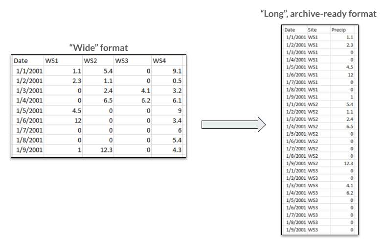
The first is frequently called "wide", "tidy", or "matrix" style and each column represents a single measured variable with each record (or row) representing one observation time and location. This format is generally preferred by statistical applications and is best described with EML metadata.

The "long" table format is characterized by having very few columns, typically a column for a location, a sampling time, one that holds all variable names and one that has the corresponding value (i.e. a key-value format). This format is preferred for maximum flexibility in adding variables at any time and avoiding many empty cells. For example, a measurement being added five years into a study would create five years of empty cells in an existing dataset.

Below is an example of "wide" and "long" formatted tables. The wide table contains precipitation data measured at four watersheds through time. The long table has each variable occupying a single column and each observation as a single row.

New measurement variables can be added as columns or within a single column as key-value pairs, where one column represents the measurement variable and its attributes are listed in adjacent columns (e.g. unit, precision).

Data table aggregation

Data can be published as a set of tables or in aggregate as a single table. For instance, time series data could be split into files by year or by variable.

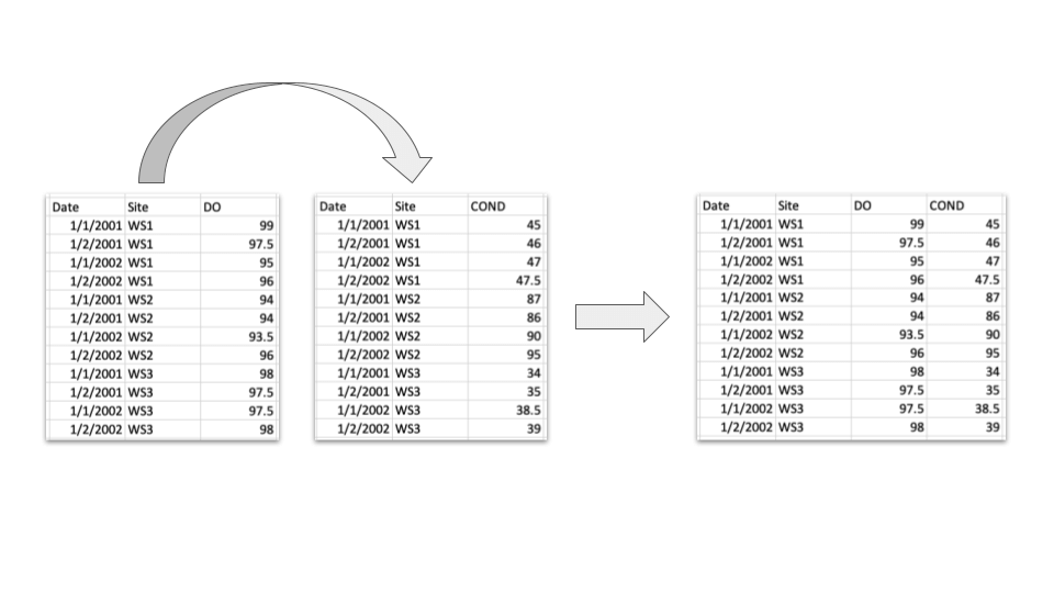
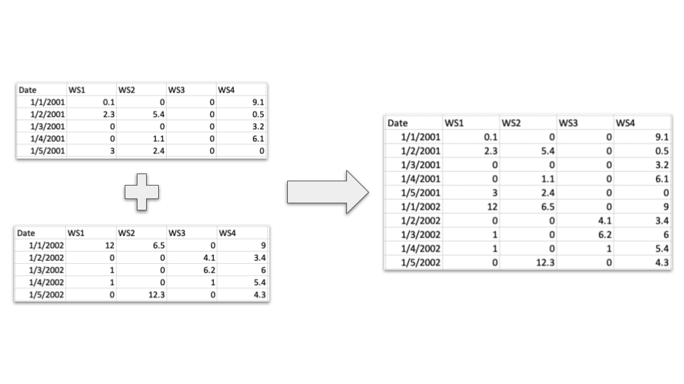
Consider who will likely be using the data in the future and what format will be simplest for them to access, understand, and work with. If the data are split, try to maintain a consistent format so the tables can either be joined by key columns or "stacked" together:

In general, a single aggregated table simplifies understanding and use rather than data split into several smaller increments. However, table splitting should be considered to simplify access and download when the data become large (e.g. in the tens of gigabytes).

One value per cell

Within a column each cell should contain only one piece of information in a consistent format to enable accurate variable typing (e.g. datetime, numeric), reshaping, subsetting, and other transformations (e.g. joins). The most frequent problems are comments entered into an otherwise numeric column (e.g. to denote a missing value). In that case it is recommended to have the value column and add a comment column where the text comments may be entered.

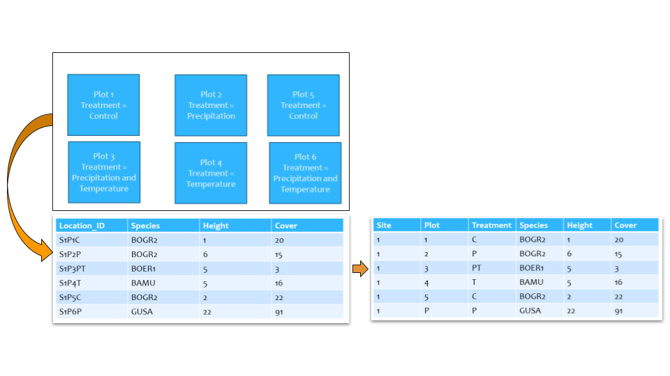
Another recommendation is to avoid overloading a cell with composite information. Below is an example illustrating the issue of more than one piece of information per cell. In the first table, the Location_ID column is a composite of multiple variables. Selecting values from a variable requires parsing. The second table follows the best practice of one piece of information per cell, where the data are easily accessed.

Variable types

Consistency within variables facilitates type wise operations allowing similar types of data to be combined and operated on together. Data become much more difficult to understand and use when variable types are mixed (e.g. numeric data mixed with character strings).

Dates and times

Using a widely accepted and unambiguous datetime format maximizes the readability across software applications and integration with other data. The EDI Data Repository recommends the ISO 8601 Standard whenever possible (e.g. YYYY-MM-DD hh:mm:ss). The full list of ISO 8601 permutations recognized by the EDI Data Quality Checker is available here. Remember to also specify the time zone and daylight savings observation practices during measurements.

Numeric

Numeric types should be consistent within a column (e.g. integer, real). If the measurements have a practical precision, the values within the column should be consistently represented in this precision, (i.e. keep meaningful numbers of decimals).

Categorical

Categorical variables are frequently used for grouping data (e.g., experimental manipulation vs. control). Check for consistent representation in terms of spelling, abbreviations, casing, synonyms, etc.

Character

Character types should only be used when the other types don't apply. Numeric values should not be character type unless, possibly, the values represent identifiers and should not be used for calculations. In many cases character fields need to be surrounded by double quotes to avoid misinterpretation of commas or apostrophes. A common issue in character data is the incomplete closure of the field with quotes, where a leading or closing quote is absent.

Missing values

Missing value codes denote when no observation was made. This differs from when data were collected and their quantity is zero. Applying consistent missing value codes within a table greatly simplifies reading into a software application. Although not strictly necessary, empty cells should be filled with a missing value code to prevent software applications from interpreting these values differently, and to enable description within EML metadata. However, every analytical software has its own prefered empty cell code.

File format

Published data should be in a non-proprietary and non-binary format. Proprietary and binary formats (e.g. MS Excel and Word), and their versions, are much less persistent and widely used than open formats (.csv, .txt). Proprietary binary formats are acceptable if they represent a community standard with open source software able to read them (e.g. several spatial data formats) otherwise the data should be exported to a non-proprietary format for publication.

Quality Control of measured values

Quality Control (QC) occurs after the data are generated and tests whether they meet requirements for quality outlined by end users, which can vary among different user groups. Therefore, it is important to publish data in a minimally processed form that preserves the originally measured values as much as possible. To do this, while providing valuable insights into potential data issues, it is common to use data flagging or data processing levels. Either way, any alteration of the values and associated rational should be clearly described in the methods section of the data package metadata.

Checking values

Value checking is implemented as tests designed to address issues likely to be present in the collected data. Some examples:

Duplicate records - Measurement listed twice. Not a replicat measurement.
Sequential records - Some data should be in a sequential order (e.g. dates and times).
Range - Data out of range may indicate a faulty measurement (e.g. relative humidity 0 - 100%).
Persistence - Constant values may indicate a faulty measurements
Slope change and steps - In time series, these may represent instrument drift.
Internal consistency - Data values fall within an established range at a sampling location (e.g. a list of species expected at a site)
Paired consistency - Duplicate observers/instruments produce similar values and trends.

Data flagging

Data flags are useful in communicating value specific information from quality control results (e.g. a value is below a detection limit or is questionable). Data flags can be added to a table as new columns using the naming convention <variable>_flag (e.g. temperature_flag).

For consistency, consider making a comprehensive set of codes to be used across all the data created by a project.

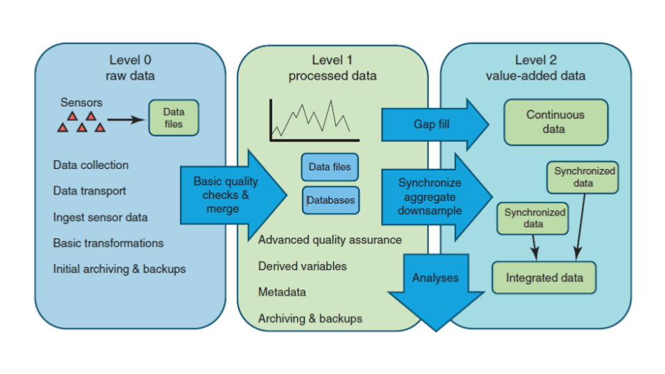
Data processing levels

Data can be processed at progressive levels and published as separate but related data packages. For example, the raw or minimally processed data can be published as a level-0 data package, and a level-1 version, with more processing applied, published as another data package. This process repeats for each new level with provenance metadata describing the relationships among the levels.

Quality Control as a process

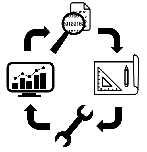
Data quality improvement is an ongoing process with the recurring steps:

Profile - Gain a quick overview of data quality in terms of outliers, maximum and minimum values, average, standard deviation, etc. Data should be profiled at the frequency of updates. Automate this as much as possible.
Design - Rules by which the data must comply and routines that modify the data. Create rules that address actual issues. Generalize the rules as much as possible to be used in other contexts. Set priorities.
Implement - Translate rules into code and implement in scripted workflows. Capture exceptions to the rules and report to the information manager.
Monitor - Track data health and report to data users. Data quality should improve. Gather user feedback.

New versions of a data package are clearly marked with an incrementing version number and should be accompanied by release notes in the metadata to communicate what has changed and why (e.g. implementation of new tests to improve coverage).